Radar Signal Processing

Produce Range-Doppler and/or Range-Angle heat maps and/or IQ Data using the same algorithms that FMCW or pulse radar equipment would use, to visualize the effects of limitations in such algorithms and/or optimize the parameters in such algorithms.

FMCW Radar Signal Processing

To obtain such a heat map and/or IQ Data, do the following:

In the results tree, select Power (MS) or Power. These are the power received by the receiver antenna and the power received by a hypothetical isotropic antenna, respectively.
Click Display > Radar > FMCW Radar.
Click on the radar result pixel.
On the FMCW Radar Postprocessing dialog, specify the parameters.

You can specify the radar parameters using two modes, either with Set Radar Parameters or Design Radar Parameters.

In case uncorrelated superposition of rays is specified in the simulation setup, the power values are summed. As a consequence, in the FMCW heatmap, the peaks are higher and the ghost targets are lower than in the case of coherent superposition.

Figure 1. If uncorrelated superposition of rays is specified in the simulation setup, the power values are summed. The peaks are higher and the ghost targets are lower (top image) than in comparison to the case of coherent superposition (bottom image).

Set Radar Parameters

You can specify the following radar parameters:

Chirp duration

The sawtooth chirp sweep period in μs. It has an impact on the maximum measurable velocity and on the velocity resolution¹ of the radar.
Sweep Bandwidth

The difference between starting and final frequency of a chirp. It has an impact on the maximum measurable range and on the range resolution² of the radar.
Number of Chirps

The number of chirps in one frame. It has an impact on the velocity resolution.
Frequency Bins

The number of FFT samples in one chirp. It has an impact on the maximum detectable range.

Design Radar Parameters

You can specify performance quantities like the desired range, range resolution, maximum velocity, and velocity resolution. It will calculate/design the radar parameters (for example, chirp duration, sweep bandwidth, number of chirps, and FFT samples) that can satisfy the required performance quantities.

Output

You can specify the desired output and optionally the type of windowing function. Windowing functions are applied in the time domain to suppress the side lobes in the frequency domain. They are also used to detect low signals that could be hidden beneath the side lobe of another target.

The output options are:

Doppler-Range:
- Heat Map
  
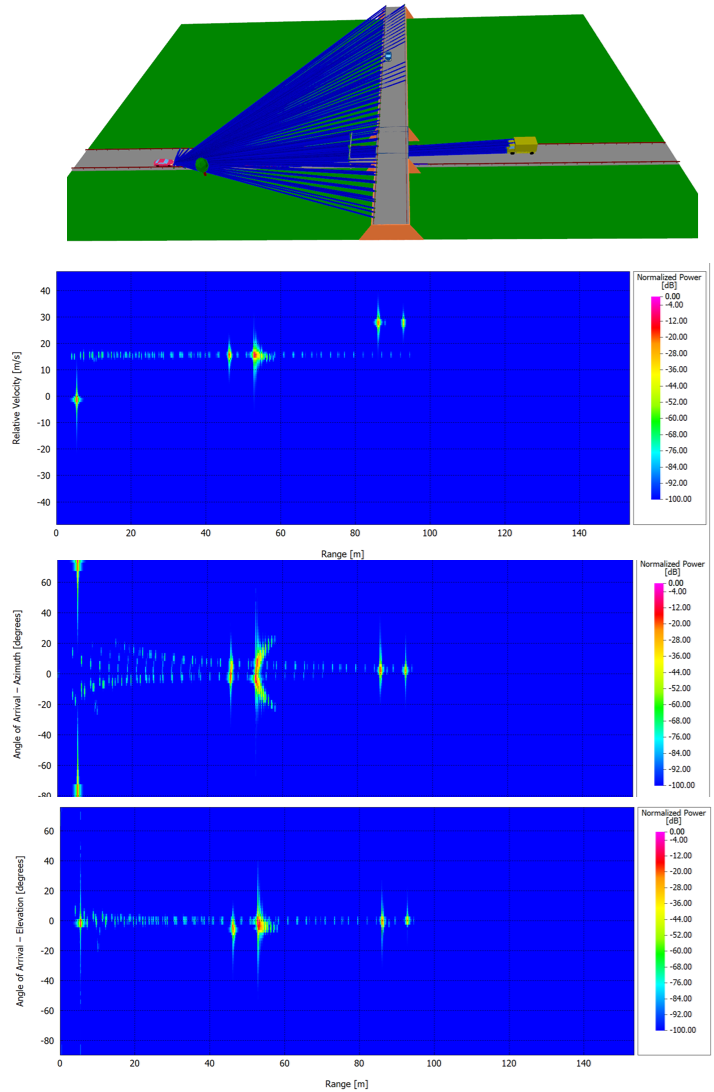
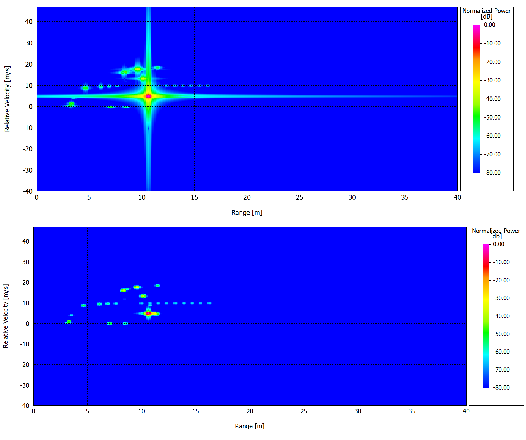
  Shows the FFT-based processed signal as a function of range and Doppler, with targets appearing as peaks in the Doppler-range map.
- CFAR (Constant False Alarm Rate)
  
  A detection map that identifies targets based on adaptive thresholding applied in the Doppler-range domain. See CFAR settings.
Angle-Range
- Heat Map
  
  Shows the FFT-based processed signal as a function of range and angle of arrival (AoA), with targets appearing as peaks in the angle-range map.
- CFAR (Constant False Alarm Rate)
  
  Similar to Doppler-Range CFAR, but applied over angle and range for detecting targets in the angle-range domain. See CFAR settings.
- MUSIC Spectrum
  
  Provides high-resolution angle of arrival (AoA) estimation using the MUSIC (Multiple Signal Classification) algorithm.
- MUSIC CFAR
  
  Applies CFAR detection on the MUSIC Spectrum to identify targets in the angle-range domain. See CFAR settings.
IQ Data
- Raw in-phase and quadrature (IQ) data captured at the Analog-to-Digital Converter (ADC) of the radar, enabling further external or custom DSP analysis. If IQ Data is selected, an ASCII file will be generated in the following format: Tx index, Rx index, Chirp, Sample, Re{IQ_DATA}, Im{IQ_DATA}.
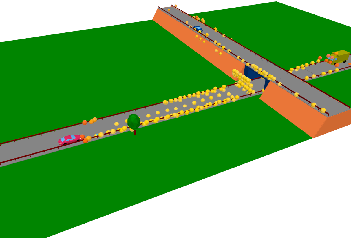
Point Cloud
- Represent detected target as a set of discrete points in the 3D view, with each point corresponding to a detected reflection, and the color of the point indicates the target velocity. Detections are determined based on the CFAR settings. Generating the point cloud requires angle estimation in both domains, azimuth and elevation. See Angle of Arrival in Azimuth and Angle of Arrival in Elevation.
  In addition to the 3D visualization, an ASCII file will be generated, listing the points relative to the sensor in the following format: Index, Range [m], Velocity [m/s], Azimuth [°], Elevation [°].
  CFAR Settings
  CFAR (Constant False Alarm Rate) is a widely used algorithm in radar systems for target detection while minimizing false alarms. It adaptively determines a detection threshold based on the surrounding noise. Multiple CFAR detection modes are supported:
  
  Cell-averaging CFAR: Estimates noise by averaging power from all reference cells. It is suitable for most detection scenarios.
  
  Greatest-of cell-averaging CFAR: Uses the higher average from leading or lagging reference cells to set the detection threshold. It can mitigate false alarms at the clutter edge.
  
  Smallest-of cell-averaging CFAR: Uses the smaller average from leading or lagging reference cells to set the detection threshold. It can reduce the masking effect caused by nearby strong targets.
  
  Order statistic CFAR: Sets threshold based on a selected rank-ordered sample among the reference cells.

For the angle of arrival estimation heat maps, note that it requires selecting one of the Power Sub-Channel results and following the same steps described above in FMCW Radar Signal Processing. The following requirements need then to be satisfied:

Angle of Arrival in Azimuth:

Multiple Receiving Antenna Elements:
- The receiver antenna type must be a Uniform Linear Array with more than one receiving element.
- The array azimuth angle needs to be set correctly, for example, in case of simulating an automotive radar, the antenna array must be aligned horizontally with the radar car's bumper.
- The horizontal spacing between the Rx elements should be $= \frac{λ}{2}$ ( $\frac{λ}{2}$ corresponds to the maximum angular field of view ±90°, where $λ$ represents the wavelength).
To obtain an accurate angle estimation, the following recommendations apply:
- Use a large number of Rx elements. For N receiving elements (with antenna spacing of $d = \frac{λ}{2}$ ), the angular resolution (for FFT-based estimation) can be approximated as follows: $θ_{r e s} \approx \frac{2}{N} [rad]$ .
- Apply a window function to reduce the ripples caused by zero padding in the angle-FFT. The angle-FFT was processed using zero-padding to improve the angle estimation accuracy.
- Use a project based on Standard Polarimetric Analysis rather than Full Polarimetric Analysis, see Set Up a New Project.
Multiple Transmitting and Receiving Antenna Elements:
- The transmitter and receiver antenna type must both be a Uniform Linear Array with more than one element.
- Same alignment requirement as above.
- For N transmitting and M receiving antenna elements, users can create (with a proper antenna configuration) a virtual antenna array of N*M elements. This leads to a multiplicative increase in the number of virtual antenna elements, resulting in improved angular resolution. The maximum angular resolution can be approximated as $θ_{r e s} \approx \frac{2}{(N \times M)} [rad]$ .
- The arrangement of transmitting and receiving elements should produce phase shifts of [0, ω, 2ω, …], and this can be accomplished using different physical antenna configurations that lead to the same virtual antenna array.
  Figure 2. Here is an example of the configurations that lead to a virtual array of 8 virtual elements, each spaced by a distance of d.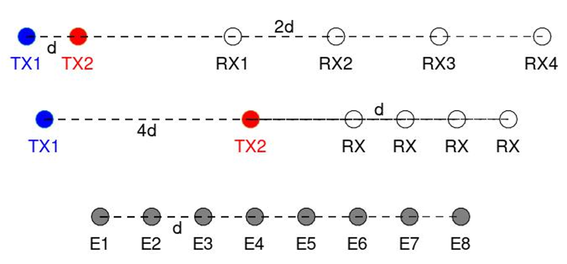

Angle of Arrival in Elevation:

The same requirements described in Multiple Receiving Antenna Elements and Multiple Transmitting and Receiving Antenna Elements apply. The key difference is that the antenna type must be a Rectangular Linear Array to provide both horizontal and vertical antenna elements. Selecting the Angle-Range check box will enable estimation of both azimuth and elevation angles of arrival.

If a heat map is chosen, it will be plotted. If IQ Data is selected, it is written to disk in ASCII format for external signal processing.

Figure 3. A snapshot in a time-variant simulation and an example of a heat map produced by FMCW processing. The first heat map shows not only the range and relative velocities, but also the artifacts produced by the signal processing algorithm with user-defined parameters. The middle heat map shows the Angle of Arrival in the azimuth domain, while the last heat map shows the Angle of Arrival in the elevation domain.

In addition to heat map visualizations, the radar can output a point cloud (if both azimuth and elevation angle of arrival estimation are available), where each detection is mapped to a 3D point in space, enabling 3D visualization of detections. The detection results displayed in the point cloud depend on the configured CFAR settings.

Figure 4. Radar detections visualized as a 3D point cloud.

¹ Velocity resolution is the ability to resolve two objects having close velocities (they show up as two peaks in the heat map).

² Range resolution is the ability to resolve two closely spaced objects (they show up as two peaks in the heat map).