Since version 2026, Flux 3D and Flux PEEC are no longer available.
Please use SimLab to create a new 3D project or to import an existing Flux 3D project.
Please use SimLab to create a new PEEC project (not possible to import an existing Flux PEEC project).
/!\ Documentation updates are in progress – some mentions of 3D may still appear.
Isotropic / anisotropic soft material: analytic saturation curve + knee adjustment
Presentation
This model defines a nonlinear B(H) dependence for an isotropic material, taking the saturation and control of the corresponding knee into consideration.
Mathematical model
This model consists, like the previous one, of a combination of a straight line and a curve. A coefficient allows for the adjustment of the knee shape in order to better approximate the experimental curve.
The corresponding mathematical formula is written as follows:
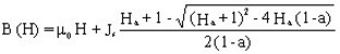
with ![]()
where:
- μ0 is the permeability of vacuum, μ0 = 4 π 10-7 H/m
- μr is the initial relative permeability of the material (at the origin)
- Js is the magnetic polarization at saturation (T)
-
a is the adjustment coefficient of the B(H) curve knee (a > 0 and a ≠ 1)
The smaller the coefficient, the sharper the knee is.
The shape of this B(H) model is given in the figure below.

Anisotropic material
For an anisotropic material, this model consists in a set of three equations, one per 3D-space direction.
This model is available when the following conditions are satisfied:
- 2D applications (2D plane domain): Magneto Static / Transient magnetic
- regions: magnetic non conducting, solid conductor